The Nature of Evidence

A lighthouse flashes six times. Another lighthouse flashes the same six times, in the same colors, over four times as long. Your notebook contains identical observations. Your experience of the two lighthouses is completely different.

Something happened between the entries.

That something is the beginning of a much larger picture of evidence. A silent alarm, an unanswered message, an empty telescope image, and a machine that has stopped reporting all contain intervals during which something could have arrived. An observer lives inside those intervals. What it learns depends on what it expected to happen there.

Miraia Chiou’s starting question was wonderfully concrete: what if the difference between the clock of arriving evidence and the clock on the wall is itself evidence? Follow that idea far enough and time becomes part of the data, silence starts exerting a force, and the bookkeeping of a belief begins to resemble the geometry of physics.

Two watches for one stream

Imagine a receiver that records support and opposition as teal and rose flashes. Its content ledger is a Beta distribution,

$$\alpha ={\alpha }_0+n_{+},\beta ={\beta }_0+n_{-},\mu =\frac{\alpha }{\alpha +\beta }.$$

Here $n_{+}$ and $n_{-}$ count the two kinds of trial, the positive quantities ${\alpha }_0,{\beta }_0$ describe the prior, and $\mu$ is the posterior mean probability of a support flash. The trial watch $A=\alpha +\beta$ advances by one whenever a unit trial arrives. A second watch records live exposure $T$: how long the receiver was able to observe.

Three support flashes and three opposition flashes turn a $\mathrm{Beta}(1/2,1/2)$ prior into $\mathrm{Beta}(3.5,3.5)$. That is true whether they arrive in three seconds or twelve. The rate estimates, however, are two flashes per second and half a flash per second. The content ledger has preserved one fact and discarded another.

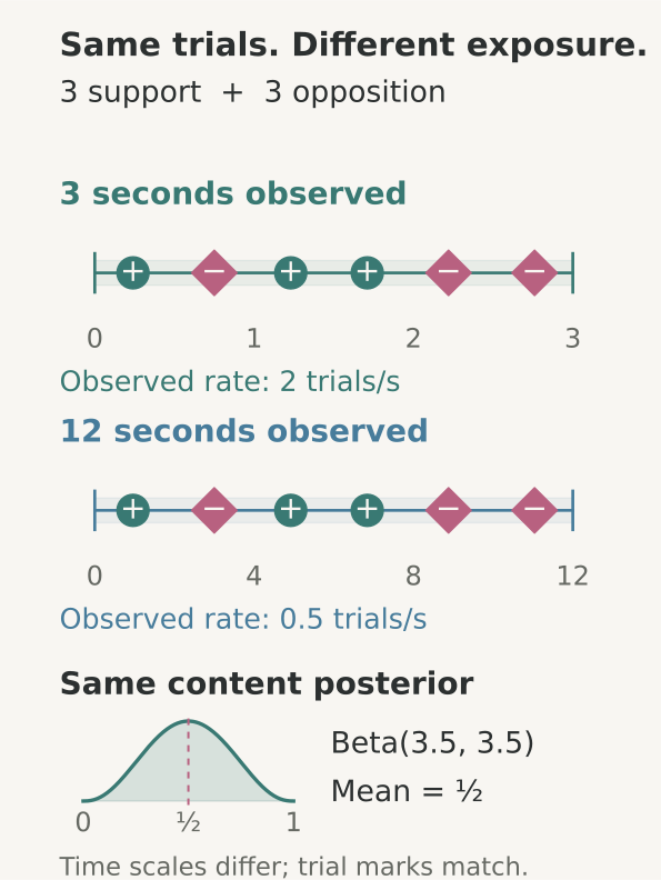
The simplest emission model is a Poisson process: arrivals occur independently at a constant rate $\lambda$. Over exposure $T$, the expected count is $\lambda T$. In symbols,

$$N(T)\sim \mathrm{Poisson}(\lambda T),\frac{d\mathbb{E}[N(T)]}{dT}=\lambda .$$

The count watch jumps; the exposure watch moves continuously. Their relationship measures how luminous the source looks to this observer. In a conversation it might measure responsiveness. In a laboratory it measures event production. In an institution it might measure how often reality manages to reach the reporting system.

Silence exerts a force

Let a hidden beacon be either bright, emitting at ${\lambda }_B=3$ flashes per second, or quiet, emitting at ${\lambda }_Q=1$. Give the two possibilities equal prior probability and identical color distributions. Only their timing differs.

The probability of seeing no flashes during exposure $T$ is $e^{-\lambda T}$. Compare the two hypotheses:

$$\frac{P(N=0\mid B,T)}{P(N=0\mid Q,T)}=\frac{e^{-3T}}{e^{-T}}=e^{-2T}.$$

Every silent second divides the bright-to-quiet odds by $e^2$. Nothing arrives, yet the belief moves.

Now include arrivals. Let $L$ be the natural logarithm of the bright-to-quiet posterior odds. After $n$ flashes and exposure $T$,

$$\boxed{L=n\log 3-2T.}$$

That one equation describes a landscape with two kinds of motion. Each flash gives an upward kick of $\log 3$. Between flashes, silence pushes downward at two log-odds units per second. If half-log-odds plays the role of rapidity, the observer is being driven through belief space by a steady field.

Call this the dark current of inference. The silence between observations has direction and strength.

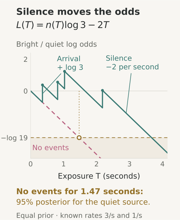
For the quiet beacon to have posterior probability $0.95$, its odds must be $19:1$. Starting from equal odds, a completely silent record reaches that point at

$$-2T_{\ast }=-\log 19,\boxed{T_{\ast }=\frac{\log 19}{2}\approx 1.4722\text{ seconds}.}$$

This also proves that no record in this setup reaches the quiet threshold sooner: every flash adds a positive $\log 3$ and delays that crossing. The game below lets you inspect the proof as a sequence of moves. Watch what happens when the receiver spends part of its journey offline.

The two-clock lookout

Listen for the hidden lighthouse

Restart watch

One lamp is hidden in the fog. Listen until one model reaches 95%, then tap that lamp to file your report.

The fog bankWatch 1 of 3

Detected n0

Live exposure T0.00 s

Wall time t0.00 s

Bright lamp3 flashes / second50.0% Quiet lamp1 flash / second50.0%

Listen · 0.50 s

The lamps start equally likely. Their flashes look identical; their rates differ.

Read the two ledgers

The model assumes independent Poisson arrivals at known rates, equally likely lamps, identical flash content, and a recorded live-sensor schedule. The count clock advances by ΔA = n; T records how long we could observe.

$$L=\log \frac{P(\text{bright}\mid n,T)}{P(\text{quiet}\mid n,T)}=n\log 3-2T$$ $$P(\text{bright}\mid n,T)=\frac{1}{1+e^{-L}}$$

Each detected flash adds log 3. Each live second subtracts 2. The graph uses wall time horizontally, so an offline interval is flat. With zero flashes, the quiet model reaches 95% after log(19)/2 = 1.4722 seconds of live exposure.

These saved tracks isolate those three moves. Count-clock advance and elapsed physical time are distinct quantities.

A smoke alarm makes the everyday version vivid. The reassuring observation is a working detector spending time without a signal. A disconnected detector has accumulated a different kind of history. This suggests a basic faculty of intelligence: keep track of whether the world was quiet, or whether you stopped listening.

What happened, and how often?

A flash can carry a mark: a color, a word, a particle type, a measurement category. Suppose hypothesis $c$ emits at total rate ${\lambda }_c$, and gives each arrival mark $w$ with probability $f_c(w)$. Over live exposure $T$, the class-dependent part of the stream likelihood is

$$P(\text{record}\mid c,T)\propto e^{-{\lambda }_{c}T}{\lambda }_c^n\prod _{j=1}^n{f}_c(w_j).$$

This is the marked point-process likelihood. Taking logarithms places the two watches beside each other:

$$\log P(\text{record}\mid c,T)=\underset{\text{what arrived}}{\underbrace{\sum _{j=1}^n\log f_c(w_j)}}+\underset{\text{how much arrived during exposure}}{\underbrace{n\log {\lambda }_c-{\lambda }_{c}T}}+\text{constant}.$$

There is a short proof hiding inside the formula. Each mark-specific count $n_w$ has Poisson mean ${\lambda }_c{f}_c(w)T$. Multiply their Poisson probabilities. Their exponential factors combine to $e^{-{\lambda }_{c}T}$ because $\sum _w{f}_c(w)=1$; their powers of ${\lambda }_c$ combine to ${\lambda }_c^{\sum _w{n}_w}$. Everything else goes into the content product or a class-independent factor.

Conditional on the total count $n$, the mark counts have a multinomial distribution. This is the familiar world of multinomial naive Bayes. Restore the probability of the total count over exposure, and it gains a second instrument. Spectroscopy asks which colors arrived. Photometry asks how much light arrived while the shutter was open.

The notebook’s seeded experiments make the distinction tangible. AUC measures ranking quality: $0.5$ is chance, and $1$ is perfect separation in the tested sample.

These runs used 20 mark channels and 3,000 training plus 3,000 test streams per class, with seed 20260919. The full numerical receipt also records the silence, burstiness, background-change, and staleness experiments.

Think of two factories sending identical reports. One sends a report after every incident. The other sends one after every hundred incidents. The wording might match perfectly while their brightness carries the distinction you care about. Or imagine a classifier that reads a document alongside how long it took to produce it. The same sentence can be a leisurely composition or a burst from an automated process. Time supplies another axis along which generators become visible.

The empty ticks become an exposure ledger

How should a receiver learn an unknown rate? A Gamma distribution gives a compact answer. Write $\mathrm{Gamma}(a,b)$ with shape $a$ and rate parameter $b$, so its mean is $a/b$. With positive prior shape $a_0$ and prior rate $b_0$, observing $n$ arrivals over live exposure $T$ gives

$$\lambda \mid n,T\sim \mathrm{Gamma}(a_0+n,b_0+T),\mathbb{E}[\lambda \mid n,T]=\frac{a_0+n}{b_0+T}.$$

This is Gamma-Poisson conjugacy. The two update rules almost look like two columns of a notebook: arrivals add to the top, exposure adds to the bottom. Silence keeps writing in the exposure column.

We can reach this rate ledger directly from the familiar Beta ledger. Chop a fixed exposure $T$ into $N$ tiny ticks, with success probability $p=\lambda T/N$ per tick. Start with a fixed $\mathrm{Beta}(r,s)$ prior. After $n$ occupied ticks, the posterior is $\mathrm{Beta}(n+r,N-n+s)$. Re-express it as a density for $\lambda$:

$$p_N(\lambda \mid n)\propto {\lambda }^{n+r-1}{(1-\frac{\lambda T}{N})}^{N-n+s-1}.$$

As the ticks become finer,

$${(1-\frac{\lambda T}{N})}^{N-n+s-1}⟶e^{-\lambda T},\lambda \mid n⟶\mathrm{Gamma}(n+r,T).$$

The countless empty ticks have condensed into a finite exposure $T$. This is an appealing picture of a continuum: refine the calendar until its individual boxes disappear, while preserving what the elapsed interval taught you. Choosing $r=1/2$ gives the posterior associated with the Poisson Jeffreys weighting $\pi (\lambda )\propto {\lambda }^{-1/2}$ after positive exposure.

The geometry also becomes simple. At fixed exposure, the Poisson Fisher metric, which measures local statistical distinguishability, is

$$d{s}^2=T\frac{d{\lambda }^2}{\lambda }.u=2\sqrt{\lambda }\Rightarrow d{s}^2=Td{u}^2.$$

A square-root ruler turns the rate axis into a uniform one. Square roots keep appearing in this landscape: the same algebraic family gives the evidence mass $m=2\sqrt{\alpha \beta }$. Perhaps this is a useful design principle for a future physics of observers: choose coordinates in which the price of telling nearby worlds apart becomes simple.

Turn, boost, subtract a background

Our receiver now has several ways to describe a stream. It can count it, compare it with a background, or listen for a cycle. Each description invites a different change of reference.

Turn the phase reference. A rhythmic sensor accumulates arrows $e^{i\omega t_j}$ from arrival times $t_j$, where $\omega$ is angular frequency. Shift every timestamp by $\mathrm{\Delta }$, and the arrow sum rotates through $\theta =\omega \mathrm{\Delta }$. In real coordinates this is

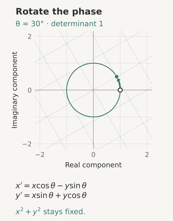
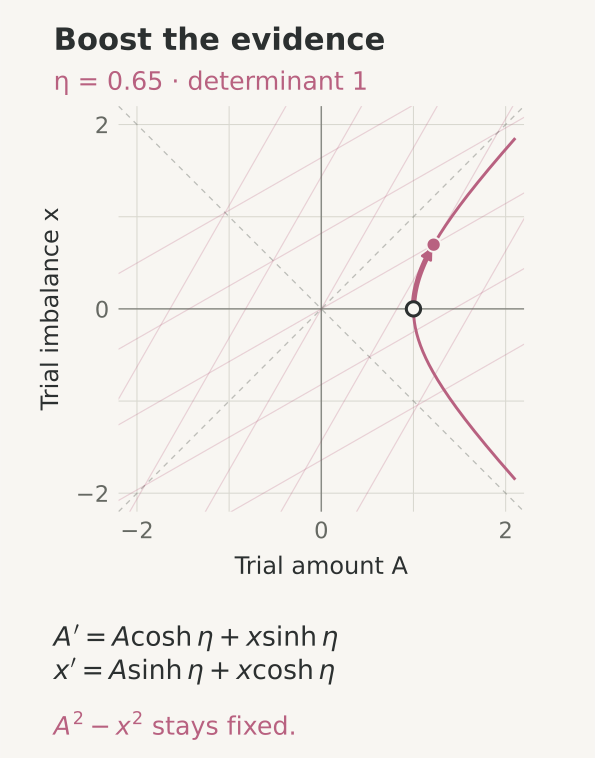
Boost the interpretation. In a Beta ledger, let $A=\alpha +\beta$ and $x=\alpha -\beta$. Reweight the two channels by $\alpha \mapsto e^{\eta }\alpha$ and $\beta \mapsto e^{-\eta }\beta$. The resulting transformation is

The parameter $\eta$ is rapidity: it adds when boosts combine. Here a hyperbola plays the role that the circle played for rotation.

Subtract a background. Suppose the receiver records a centered count $q=n-{\lambda }_{0}T$, measuring arrivals above a reference rate ${\lambda }_0$. A second observer chooses ${\lambda }_0+\delta$. Their description is

This is the same form as the Galilean coordinate change $x^{\prime }=x-vt$, $t^{\prime }=t$. A background rate behaves like a reference velocity. Two astronomers can disagree about the baseline and still agree on the exposure and the raw photons.

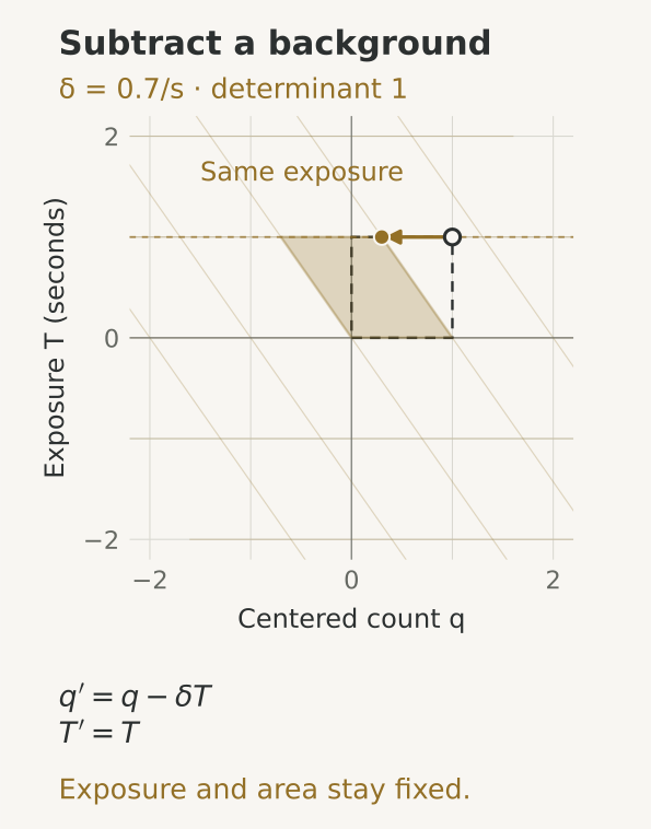
Now try these moves as a small navigation game. The same operation cards appear in both plots; reversing their order reveals how a sequence of interpretations can acquire its own geometry.

The order of a frame change

Fit the constellation

Reset game

Challenge 1. Turn the telescope2. Choose the order3. Arrange all threeExplore freely

Move the constellation into the gold rings with one turn.

Choose a card below

Turn quarter turn Stretch diagonally Shear sideways

Undo

Tap a colored card to move the stars.

Hint and the matrix connection

Turn moves every star a quarter-circle counterclockwise around the origin.

Here (x, y) are geometric coordinates. Each card acts on their column with a real matrix:

Turn R(θ)cos θ−sin θsin θcos θθ = π/2

Stretch B(η)cosh ηsinh ηsinh ηcosh ηη = ln 2

Shear H(s)1s01s = 1

All three have determinant 1, so they preserve oriented area. Applying A first and B second gives BA. The same operation cards can therefore have different effects in a different order.

Your full map1001det = 1
Δ = 0

The trace tr M is the sum of the diagonal entries. The discriminant Δ = (tr M)² − 4 det M is negative for elliptic maps and positive for hyperbolic maps. Zero includes nontrivial parabolic shears and scalar maps such as the identity. Your current map is scalar.

In the evidence connection, a phase reference turns, a boost mixes two coordinates, and changing a background rate shears (centered count, exposure). This game compares their geometry on one shared plane.

Three motions, four knobs, many worlds

There is a satisfying piece of algebra underneath the pictures. Let $I$ denote the identity matrix, and define

Multiplying them gives $J^2=-I$, $K^2=I$, and $JK+KJ=0$. Their exponentials generate turns and boosts. A shear generator is already waiting inside the pair:

Because $N^2=0$, the entire exponential series stops after its linear term: $e^{sN}=I+sN$. A parabolic move emerges from a combination of the circular and hyperbolic generators.

This is where an adventurous reading becomes irresistible. Phase, interpretation, and baseline could be three ways an observer negotiates its relationship with a stream. The operations can interfere through their order, just as turning and walking interfere when you navigate a room. A mind might carry a geometry of how it changes its interpretation, alongside the beliefs themselves.

For a general traceless real generator

the sign of $a^2+bc$ gives circular, hyperbolic, or nonzero nilpotent motion. The zero generator gives no motion. This is a compact proof of the three signatures within this two-dimensional linear setting.

Add an overall positive scale, and every real $2\times 2$ matrix $M$ with positive determinant can be written

This is the Iwasawa factorization with scale included. The diagonal factor is a boost in light-cone coordinates. We have four knobs: scale, phase, reciprocal gain, and shear. That is an intriguing blueprint for a compact observer. Its architecture could consist of many such little question-planes, each carrying a local reference and exchanging evidence with its neighbors. The complex, dual, and split-complex algebras give a mathematical companion to these three signatures.

A ledger is a lens you choose to carry

How many of those planes should an observer carry? Consider the transform

$$S(z,w)=\sum _{j:w_j=w}{u}_j{e}^{z{t}_j},$$

where $u_j$ is an event weight and $z$ selects a way of looking at time. Keep live exposure alongside it. The same event stream now offers several lenses:

For a fixed set of events, shifting all timestamps by $\mathrm{\Delta }$ multiplies $S(z,w)$ by $e^{z\mathrm{\Delta }}$. Imaginary $z$ rotates a response; paired real samples acquire reciprocal gains. An online implementation also injects arriving events and removes any that leave its window.

A particularly revealing experiment uses two events half a cycle apart: $1+e^{i\pi }=0$. The rhythmic response disappears while the count stays two. The observer has encountered a blind spot of its chosen lens. Where zeta waves fall silent follows this cancellation into much stranger territory.

This invites a different picture of intelligence. An intelligent system might improve by discovering which summaries it needs to keep. Counts reveal preferences, gaps reveal rates, phases reveal rhythms, and transitions reveal habits. A new concept can be a new instrument aimed at a part of experience that the old instruments averaged away.

The world dims, the channel closes, or the messages bunch

Imagine watching five bands of a spectrum. One band dims while the other four keep flowing. You might suspect a selective filter. All five go dark together, and you might suspect an outage. Keep changing the question: did the source change, did the path change, or did the receiver change?

That is also a useful way to investigate an organization. A missing category of incident reports can be an absorption line in its communication channel. Comparing independent reporting routes, sending a harmless test message, or measuring response to a scheduled check-in can make the invisible route observable. An institution could maintain a map of its own exposure: where it has eyes, when they were open, and which kinds of event could actually reach them.

In a simple channel model, the observed rate in band $w$ is the source rate multiplied by a transmission factor $h_w$. Uniform transmission reduction leaves the mark probabilities unchanged; a band-specific reduction changes their proportions. Recording exposure gives us a way to investigate brightness as well as color.

Messages also arrive in bursts. Let a document’s event rate vary according to a Gamma distribution with shape $k$; conditional on that rate, let its count be Poisson. If the mean count is $\mu$, the resulting Gamma-Poisson mixture has

$$\mathrm{Var}(N)=\mu +\frac{{\mu }^2}{k},\underset{\text{Fano factor}}{\underbrace{\frac{\mathrm{Var}(N)}{\mathbb{E}[N]}}}=1+\frac{\mu }{k}.$$

The Fano factor compares variance with mean count. A fixed-rate Poisson source has value one; this mixture bunches more strongly. The source experiment held mean rates equal and found Fano factors around $1.01$ versus $10.93$. Its classifier ranking barely moved when the burst model was added, while log loss, which penalizes poor probability assignments, improved from $2.18$ to $0.60$.

The connection to belief is intimate. Ten repetitions can belong to one burst, one copied report, or ten independent encounters. Their lineage determines what the repetition means. A good ledger remembers enough about the generator to avoid treating every echo as a new world speaking.

Forgetting can keep you in contact with the world

Now let the beacon move while the receiver hears nothing. Assume its position follows Brownian drift with variance rate $D$, meaning an unobserved interval of duration $t$ adds independent displacement variance $Dt$. If the initial position uncertainty has variance $P_0$, prediction gives

$$\boxed{P(t)=P_0+Dt.}$$

This is the basic Brownian prediction step. The proof is the addition rule for independent variances: uncertainty already present, plus uncertainty accumulated during the unseen motion. Define precision $q=1/P$. Differentiating gives

$$\boxed{\frac{dq}{dt}=-D{q}^2,}q(t)=\frac{q_0}{1+D{q}_{0}t}.$$

Precision reaches half its starting value after $t_{1/2}=1/(D{q}_0)$. No new trial is needed for a forecast to become more spread out. The outside world supplies the motion.

Try choosing a prediction band before revealing a spread of possible positions. The task is to keep a useful forecast through the silence.

The search boat

Find the drifting buoy

Restart voyages

The buoy’s radio went quiet. Choose the smallest search band that holds 90% of its predicted positions.

The moored buoyVoyage 1 of 3

Four seconds pass. The buoy cannot drift.

Your search bandLast 90% band

Radio gap 4 sNew trials 0

Close Roomy Wide

Send the search boat

Choose Close, Roomy, or Wide, then reveal the possible positions. A wider band spends more search area.

What moves during the radio gap?

The last position estimate is Gaussian, centered at zero, with variance P₀ = 0.25. Independent Brownian motion adds D units of variance per second. The radio schedule is independent of position. Here D = 0.

$$P(T)=P_0+DT,q(T)=\frac{1}{P_0+DT},\frac{dq}{dT}=-D{q}^2$$ $$\text{90\% band}=[-1.64485\sqrt{P(T)},+1.64485\sqrt{P(T)}]$$

Variance is now 0.25 and precision q = 1/P is 4.000. With D = 0.25, the initial precision halves after P₀/D = 1 second.

The 20 dots are fixed Gaussian reference quantiles, one at the middle of each 5% probability slice. They redraw the endpoint distribution at this elapsed time. The coverage percentage comes from the Gaussian distribution itself.

Think of a robot tracking another vehicle, a traveler remembering a shop’s opening hours, or a scientific community carrying an old estimate into a changing environment. An accurate memory can become an inaccurate forecast. The better you knew the starting position, the more dramatic the loss of precision can feel when the world moves beyond it.

Perhaps forgetting is partly an instrument for staying synchronized with reality. An adaptive observer could learn two rates at once: how quickly useful trials arrive, and how quickly their target drifts. Its memory would lengthen in stable terrain and shorten near a moving frontier. Curiosity could steer the shutter toward places where that mismatch is largest.

A possible physics of attention

Bring the pieces together. An observer records marks, carries an exposure map, learns the rhythm of its sources, and predicts how far the world can move during silence. It also remembers which tracelets came from the same lineage. These ingredients suggest a richer version of naive Bayes, a Wise Bayes whose object is a living stream.

Attention becomes a choice of exposure. Memory becomes a choice of weighting over time. A background model becomes a reference frame. Surprise can come from a new observation or from an expected observation failing to arrive. Learning a new concept can mean opening a new question-plane, rather than merely adding weight to an existing answer.

We could build a small artificial society around this idea. Give its members equal event budgets but different shutters, communication delays, and reference rates. Let them exchange reports with lineage attached. Then ask when they discover a common world, when they mistake echoes for consensus, and when an absence of reports becomes collective blindness. Its politics would have an observable geometry: who can see what, for how long, through which channel.

Or push toward physics. Suppose an observer’s operational time is tied to the evidence it can acquire, while its transforms describe the admissible changes of reference. Turns, boosts, shears, and the limits of observation might become the raw materials from which a physical description is assembled. The matrix identities give us something concrete to build with; the next experiment asks what sort of world those observers would discover.

The lighthouse keeps flashing. Our task is to carry a notebook rich enough to notice both its light and the space between the flashes.

Assumptions and the edge of the map. The beacon comparison uses known constant rates; the marked-stream model uses independent marks and measured live exposure. Its 95% posterior is conditional on that model, not a universal sequential error guarantee. Learned timing models can fail. Trial amount $A$ counts prior weight and arrivals; the rate derivative concerns expected counts. The Beta-to-Gamma limit fixes its prior and tick convention, with an improper limiting prior before positive exposure. Brownian prediction assumes independent drift with known variance rate $D$; its precision $q$ differs from Beta trial amount. Distinguishing source changes, channel loss, and missing observations needs calibration or intervention. The numerical results are seeded synthetic examples, and the buoy game uses fixed Gaussian quantiles. The matrix identities hold in the displayed two-dimensional representation; choosing a transform bank is part of designing an observer. The proposed connections to attention, institutions, and physics are invitations to build and test new models.